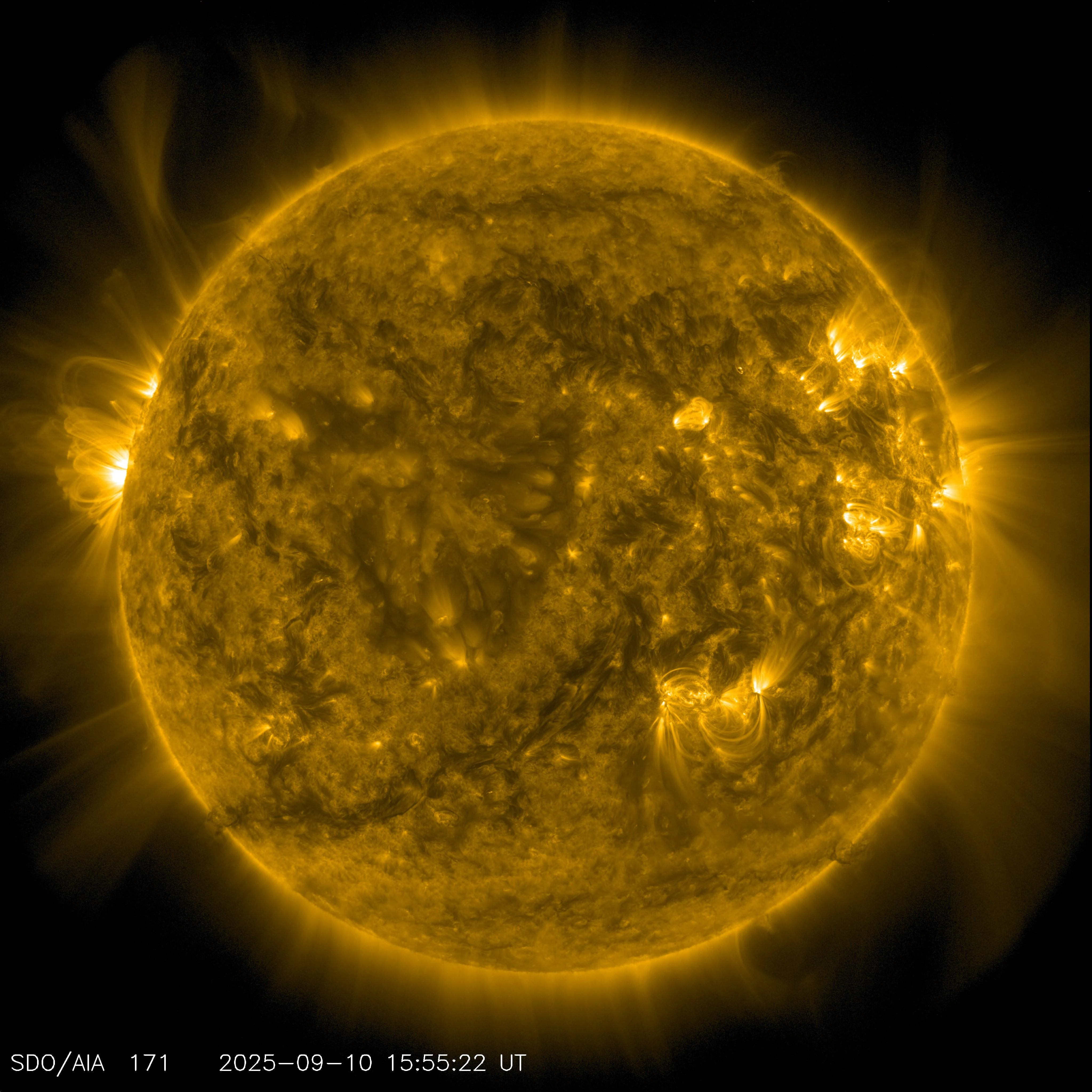
The Sun is a bell. Not a metaphor — the entire solar interior resonates with acoustic waves, trapped pressure oscillations that bounce between the surface and the core roughly every five minutes. The field that studies these oscillations is called helioseismology, and for three decades a network of ground stations has been recording every pulse.
A team at the University of Sheffield and the National Solar Observatory just ran 30 years of those oscillations through three different machine learning architectures. All three converge on the same prediction: Solar Cycle 25 peaked in early 2025, and the next minimum falls around 2030–2031. The paper, published this month in Solar Physics, is one of the first to treat the Sun’s acoustic frequency shifts as a forecasting signal for the solar cycle — not just a diagnostic one.
What p-modes are and why they shift
If you drop a marble into a bathtub, the water rings. The Sun does the same thing, except the “bathtub” is a 1.4-million-km sphere of plasma and the “marbles” are convective motions churning in the outer third of the interior.
The resulting pressure waves — p-modes, because pressure is the restoring force — propagate inward, refract off hotter and denser layers, curve back up, and hit the surface again. Each round trip takes about five minutes for the dominant modes. The Sun sustains millions of these resonant modes simultaneously, each sampling a different depth and latitude. It’s a CT scan where the probing signal is sound.
Since May 1995, the GONG network — six stations spaced around the globe so the Sun is always visible to at least one — has measured Doppler-shifted surface velocities in nine-day cadences. Each nine-day window yields mode frequencies across harmonic degrees ℓ = 0 to 100, spanning 1,500–5,500 μHz.
The key observation: those frequencies aren’t constant. They shift with the solar activity cycle. When activity rises, frequencies nudge upward. When the Sun quiets, they drop. This was established in the late 1990s. What wasn’t clear was whether you could use the pattern to predict the cycle’s trajectory, not just confirm where it’s been.
Three models, one answer
Rekha Jain, Akash Kumar, and Sushanta Tripathy applied three ML architectures to the GONG record:
Wavelet + LGBM. A discrete wavelet transform (Daubechies-4) decomposes the frequency-shift time series into trend and detail components. A LightGBM regressor then forecasts each component using temporal lag features and sinusoidal seasonality terms from spectral analysis.
LOESS-FFT + LGBM ensemble. Locally estimated scatterplot smoothing strips the trend; an FFT isolates dominant periodicities in the residual. Separate LGBM models handle trend and residual, and their forecasts are averaged.
N-BEATS. A neural basis expansion model with trend and seasonality stacks, trained on the longer proxy series — 10.7 cm radio flux and sunspot number going back to 1954 — then applied to the shorter p-mode record.
All three used an 85:15 temporal train-test split, quantile regression for 90% prediction intervals, and RMSE evaluation. The predictions diverge slightly in shape (the wavelet path descends more smoothly, the LOESS-FFT path is steeper), but they agree on timing: the frequency maximum was reached in early 2025, and the next minimum sits around 2030–2031 — a roughly seven-year descent, comparable to Solar Cycle 23.
The quadratic surprise
One result that caught my eye: the relationship between p-mode frequency shifts and the two standard activity proxies (10.7 cm radio flux and international sunspot number) isn’t linear. It’s quadratic.
At low and moderate activity, frequency shifts track the proxies cleanly. But during high activity, the p-mode response saturates — frequencies stop climbing as fast as the sunspot count suggests. The team documents this across cycles 23, 24, and the rising phase of 25.
If you built a naive linear predictor — sunspot number up by X, p-mode shift up by Y — you’d overpredict the shift at solar maximum and underpredict during the decline. The quadratic model catches that saturation and gives tighter residuals.
The physical mechanism isn’t fully pinned down. Jain and colleagues suggest it relates to how concentrated magnetic flux in active regions alters the acoustic cavity differently from diffuse flux during quieter periods. They flag it as an open question, which I appreciate.
What this means for space weather
Space weather forecasting currently depends on surface and external indicators: sunspot counts, the 10.7 cm solar radio flux, direct solar-wind measurements from ACE and DSCOVR at the L1 Lagrange point (about 1.5 million km sunward of Earth).
P-modes are different. They probe the convection zone, where the magnetic flux that eventually becomes active regions is being generated. In principle, frequency shifts could signal a change in activity before it shows up on the photosphere. Dr. Jain describes the approach as “using machine learning to listen to the acoustic heartbeat of the sun” to “track the energy drivers moving from the deep interior toward the surface and beyond.”
The team is careful to call this “a nascent step.” I think that’s honest. Thirty years of GONG data covers only about 2.5 complete cycles. The models are trained on a small sample, and predictions beyond the next few years carry wide confidence intervals.
But the direction is worth watching. ESA’s SMILE mission, which launched on May 19, is designed to study how the solar wind interacts with Earth’s magnetosphere in real time. If helioseismic ML forecasts eventually achieve multi-month lead times on solar activity phases, they’d pair well with SMILE’s X-ray imaging of the magnetopause. One tells you what the Sun is about to do; the other shows Earth’s magnetic shield responding.
What it means from my balcony
For those of us who observe, the practical takeaway is straightforward. If these three models are right, we’ve passed solar maximum. Solar Cycle 25 turned out stronger than most 2020-era predictions suggested — the “surprisingly active” stretch that solar observers have been talking about for the past year. From here, activity tapers.
By 2028–2029, expect fewer sunspot groups, fewer large flares, and — for aurora chasers at mid-latitudes — fewer Kp ≥ 5 nights. The big geomagnetic storms of 2024–2025 are probably the cycle’s peak output.
The flip side: a quieter Sun means darker skies for deep-sky work. From Troodos at 1,700 m the zodiacal light is already obvious by 04:30 local time in spring; approaching minimum it’ll only sharpen. And the next uptick, Solar Cycle 26, probably won’t start climbing until the early 2030s.
The ML pattern in solar physics
What I find most interesting about this paper isn’t the specific prediction. It’s the methodology. LightGBM and N-BEATS are commodity tools. The feature engineering — wavelets, LOESS, FFT decomposition — is textbook signal processing. The insight was pointing them at a dataset that’s been sitting in GONG’s archive for three decades, previously analyzed almost entirely with classical fitting methods.
I keep seeing this pattern across AI × astronomy. The RAVEN exoplanet classifier I wrote about earlier this month used gradient-boosted trees — nothing exotic — and confirmed 118 planets that human vetters hadn’t reached yet. Here, three off-the-shelf models decode a 30-year acoustic time series and produce a forecast that agrees with (and adds independent information to) sunspot-based predictions.
The breakthroughs aren’t coming from novel architectures. They’re coming from researchers who know their data intimately and know which ML tool fits the signal structure. The models are the easy part. The hard part is 30 years of patient, unglamorous data collection by GONG’s six stations.
The paper is on arXiv at 2604.20802, published in Solar Physics (DOI: 10.1007/s11207-026-02660-y).