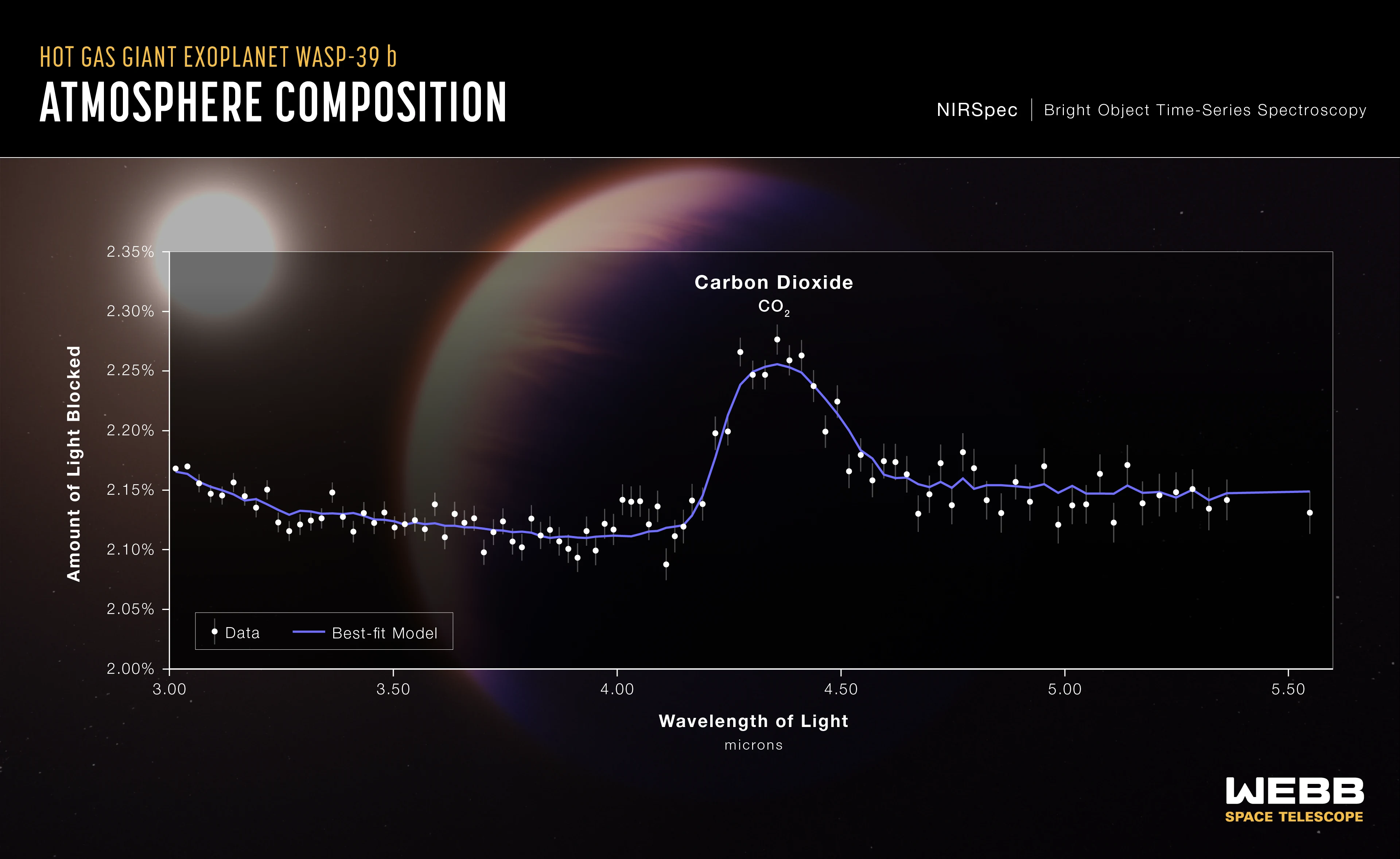
Running a full atmospheric retrieval on a JWST transmission spectrum of WASP-39b took about 498 hours of compute with standard settings, roughly three weeks of a core grinding away. A new transformer neural network gets the same answer in about 64. Same retrieval code, same Bayesian machinery, same posterior at the end. It just starts the search in a far better place.
The paper is Exoformer: Accelerating Bayesian atmospheric retrievals with transformer neural networks, led by L. Pagliaro and published in Astronomy & Astrophysics this spring. I spent years training neural nets before I started pointing a Seestar off my balcony in Nicosia, and what I like about this one is what it refuses to do. It doesn’t hand you an answer from a black box you can’t check. It speeds up the slow, principled method by giving it a good first guess.
What a retrieval actually is
When JWST “finds methane” or “detects CO₂” on a planet like TOI-199 b, it isn’t reading gases off a display. It records a transmission spectrum. During a transit, a sliver of starlight filters through the ring of atmosphere at the planet’s terminator on its way to us, and molecules there absorb at their own wavelengths. What comes back is a spectrum with dips, deeper where the atmosphere is more opaque. The measurement is the spectrum. The science is everything you do to turn that spectrum back into a temperature, a set of molecular abundances, and a radius.
That backward step is atmospheric retrieval, and it’s an inverse problem. You have a forward model (feed it a composition and a temperature, and it computes the spectrum you’d see) and you run it in reverse: search for the parameter values whose synthetic spectrum best matches the data, with error bars on each. The standard tool is a framework like TauREx driving a nested-sampling algorithm. It works. It’s also where the CPU-weeks go.
Why it’s slow
Nested sampling is a Bayesian method: it doesn’t just find the best-fit parameters, it maps the whole probability landscape and computes the evidence, the number you need to say whether a model with, say, CO₂ is genuinely preferred over one without it. It does that by scattering “live points” across the parameter space and slowly contracting them toward the high-likelihood region. Every step asks the forward model for a fresh synthetic spectrum, and a retrieval converges only after hundreds of thousands to millions of those evaluations.
The expensive part is that the sampler starts ignorant. With standard uniform priors it treats every water abundance between one part in ten billion and one part in ten as equally plausible before it looks at the data, and every temperature between 1,000 and 2,000 K, and so on across six or more parameters. Most of that box sits nowhere near the answer, and the sampler burns most of its compute learning what a person eyeballing the spectrum could have guessed in a second.
What Exoformer does
That guess is what Exoformer automates. It’s a transformer, the same architecture behind large language models, but instead of tokens of text it eats a spectrum: 515 points from 0.3 to 50 μm. Each point is embedded into a 128-dimensional vector, given a positional encoding so the network knows where in wavelength it sits, and passed through five transformer encoder blocks with eight-head self-attention. Self-attention is the useful part for spectra. It lets the network weigh how a dip at 4.3 μm relates to one at 2.7 μm, learning the correlations a molecule stamps across the whole band rather than fitting each wavelength in isolation. A couple of pooling and dense layers at the end collapse all that into six numbers: the abundances of H₂O, CH₄, CO and CO₂, an isothermal temperature, and the planet’s radius.
The team trained it on ten million simulated transmission spectra generated by the same TauREx forward model the retrieval uses, across hot-Jupiter parameter ranges. A single best-guess number is useless without an uncertainty, so they run the network with Monte Carlo dropout: 100 forward passes with dropout left switched on, each pass seeing a slightly different sub-network, and the spread across passes becomes an estimate of how confident the model is. The output isn’t a point. It’s a rough posterior.
The trick is priors, not answers
The design decision that makes this sound rather than merely fast is what happens next. Plenty of machine-learning retrieval papers stop at the network’s output and call it the answer. The trouble is you can’t fully trust those error bars: a net that regresses straight to abundances has no way to compute Bayesian evidence, so it can’t tell you whether the data actually justify adding a molecule. Exoformer instead takes its predicted posterior and turns it into an informative prior, a Gaussian centered on the network’s guess for each parameter, bounded to the same physical ranges as before, and hands that to the nested sampler as its starting belief. Then the real retrieval runs, exactly as it would have, likelihood and evidence and all. The sampler simply stops wasting weeks in the empty corners of the box, because it’s been told roughly where to look.
It’s a division of labor I’ve come to trust in scientific ML: let the network do the cheap, fuzzy pattern-matching it’s good at, and leave the rigorous, checkable inference to the method that was already correct. It’s the same instinct behind the emulators that sped up cosmology inference, and the opposite of asking a model to just hand over the result.
The numbers
On real JWST data the payoff is uneven but real. For WASP-39b, the hot Saturn where JWST made the first clear detection of CO₂ in an exoplanet atmosphere back in 2022, the retrieval on NIRSpec PRISM data dropped from 498 hours with uniform priors to 64 with Exoformer’s, a factor of 7.8. For WASP-17b, a puffy hot Jupiter observed with NIRISS SOSS, the gain was smaller: 86 hours down to 27, a factor of 3.2. The variation is the point: how much a good prior helps depends on how sharp the data are and how well the network’s guess lands.
The number that counts for more than either speedup is the one showing the answer didn’t move. Across the retrievals the Bayesian evidence shifted by less than 5 in log units, which on the usual scale means the uniform-prior and Exoformer-prior runs are statistically indistinguishable in what they conclude. You aren’t trading accuracy for speed. You’re getting the same posterior, sooner.
Where it breaks
The limitations are where the paper earns its keep. Exoformer only knows the four molecules it was trained on. It has nothing to say about SO₂, which JWST famously found in WASP-39b as a fingerprint of photochemistry, or about H₂S, TiO or VO, so for those species it can’t sharpen the prior at all and the retrieval still finds them the slow way. The training spectra were clean analytical models, while real data carry noise and instrument systematics. The wavelength grid the authors used is a holdover from the HST era and is too coarse for JWST’s resolution. Planetary mass is degenerate enough that they fixed it rather than retrieve it. And the whole thing is trained on hot Jupiters; small, cool, more interesting planets are out of scope until someone builds the training set for them.
One failure mode is worth naming. A confidently wrong prior is worse than no prior: it can steer the sampler away from the true answer, or, if it’s narrow and mismatched, actually slow convergence, the so-called “unrepresentative prior” problem. Bounding every prior to its physical range is the guardrail here, and it’s the kind of thing that will need watching as these tools scale.
Why it reaches the science you read
You’ll never run TauREx from a balcony, but the bottleneck it solves sits upstream of every JWST atmosphere headline. The telescope is producing exoplanet spectra faster than teams can wring the science out of them, and ESA’s Ariel, due around 2029, will do almost nothing but stare at roughly a thousand exoplanet atmospheres for years. Retrieval is the slow step in that pipeline, the one measured in CPU-weeks per planet. Cutting it by three to eight times is the difference between working through a backlog and keeping pace with the instrument. It’s the story I keep meeting across survey astronomy this year, from Euclid’s lens finders to Rubin’s alert brokers: the hardware got fast, and the frontier moved to trusting the software that keeps up with it.
Unlike a lot of ML-in-astronomy work, you can poke at this one directly. The Exoformer code and the TauREx plugin that feeds its priors into a retrieval are both on GitHub. When the next JWST atmosphere result lands — the next methane, the next CO₂ — there’s a fair chance a network like this one quietly took a couple of weeks off the answer.