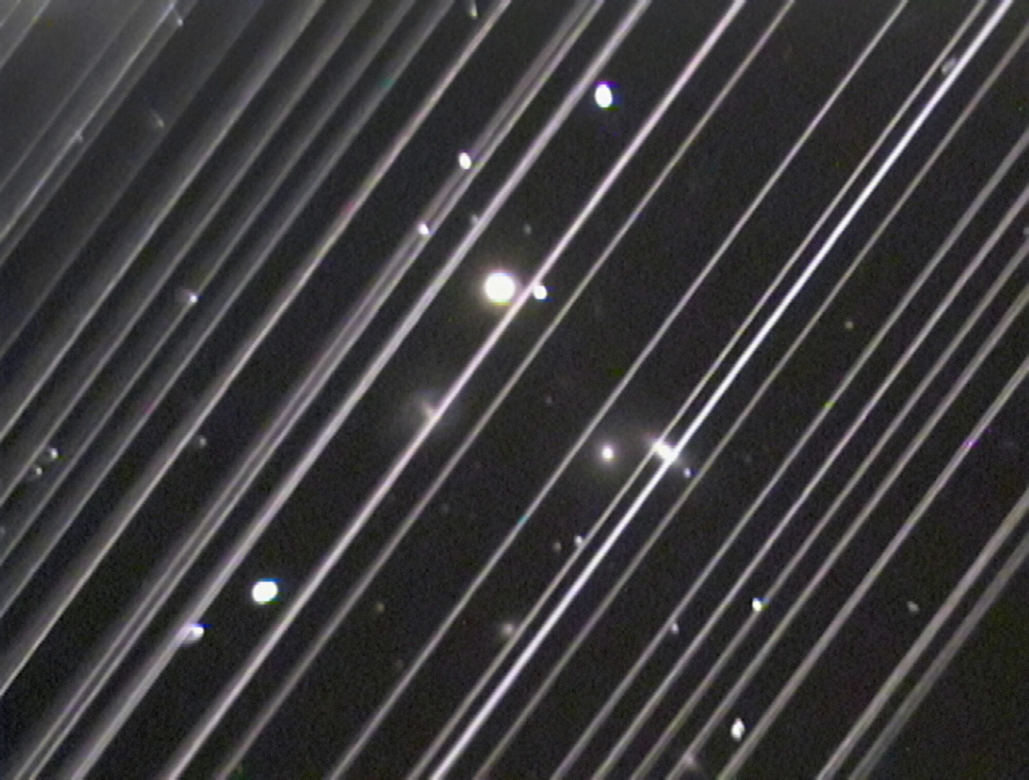
In 2023 the VLT Survey Telescope on Cerro Paranal recorded 1,246,048 CCD frames with its OmegaCAM imager. A team led by Elisabeth Rachith at EPFL ran all of them through a deep-learning streak detector, and their June 2026 preprint reports 25,335 streaks from satellites, rocket bodies and debris, with at least one in 16.9% of exposures. In the months checked by hand, about a fifth of the confirmed streaks matched nothing in the public satellite catalogue. Below: how these networks work, what the VST numbers say, and why a stack of backyard subs mostly doesn’t need one.
From my balcony in Nicosia, the Seestar S50’s 10-second subs catch trails through the first hour of every clear night, and I lose a couple of frames per half-hour session to them, as I wrote in June. Starship Flight 14 reportedly deployed the first 26 Starlink V3 satellites on 28 September (Interesting Engineering), and I haven’t found published brightness measurements for them yet. Survey astronomers aren’t waiting. They’re building software that counts the damage frame by frame.
Why a straight line is hard to find
The standard tool is the Hough transform, in the form Duda and Hart published in 1972. Describe every possible line by its angle θ and its perpendicular distance ρ from the origin, where ρ = x cos θ + y sin θ, and let each bright pixel vote for every line that could pass through it. Stars scatter their votes across the (ρ, θ) grid. The few hundred pixels of a satellite trail all vote for the same line, and that bin lights up.
It still sits inside most of the pipelines below. The trouble is that a deep image is full of other straight things. When the VST team ran their detector over real 2023 frames without a second-stage filter, the false alarms fell into four groups: bleeding columns from saturated stars, diffraction spikes, filter fringes, and a miscellaneous pile that included stray light. Siril’s documentation for its own streak detector names the amateur version: “if there is a gradient or a cloud, the bright area itself will be detected as a streak” (Siril docs). And real trails flicker when a satellite tumbles.
A neural network can learn what a trail looks like in context, and just as usefully, what a diffraction spike looks like. The groups working on this have framed it three ways.
Teaching a network what a trail is
Paint the pixels, then fit the line
ASTA (Stoppa et al., A&A 692, A199, 2024) treats the trail as a segmentation problem. A U-Net, the encoder–decoder architecture originally designed for biomedical images, takes a 528 × 528-pixel patch and outputs, for every pixel, the probability that it belongs to a trail. The authors threshold that map at 0.58 and pass the surviving pixels to a probabilistic Hough transform, which turns a fuzzy blob into a line segment with defined endpoints. The network recognises and the old geometry measures.
The data come from MeerLICHT, a 65 cm telescope in South Africa covering 2.7 square degrees at 0.56 arcseconds per pixel, usually in 60-second exposures. Training started from just 178 full-field images labelled by hand. A full 10.5k × 10.5k frame takes 4.59 ± 0.33 seconds end to end on an RTX 2080 GPU, against 23.96 seconds on the CPU.
Draw a tilted box
StreakMind (Carrillo Navarro et al., A&A 708, A211, 2026) treats each trail as an object to be boxed, using YOLO11 with oriented bounding boxes: rectangles that rotate to lie along the streak. Trained on 2,335 images mixing real frames with synthetic streaks, it reached 94% precision and 97% recall on its test set, then links detections across consecutive frames and cross-identifies them with known satellites.
The hardware caught my eye. The images come from La Sagra Observatory in southern Spain, taken with a Celestron C14 at f/2.1 through Fastar optics and an SBIG ST-10 camera at 4.12 arcseconds per pixel. That’s a commercial tube plenty of amateurs own.
Put the Hough transform inside the network
The VST pipeline goes furthest. Its detector, HT-LCNN, is adapted from Deep Hough-Transform Line Priors (Lin, Pintea and van Gemert, ECCV 2020). Feature maps from the early convolutional layers are projected into (ρ, θ) space, processed there with small convolutions that respond to lines spanning the whole patch, then projected back and merged with the ordinary image branch. The network sees local texture and global geometry at once.
Training used 384,000 hand-annotated 512 × 512 patches from raw OmegaCAM frames, seeded with 224,291 artificial streaks from a simulated population of objects 1 cm to 2 m across, on circular orbits from 300 to 36,100 km. On that set the detector scored F1 = 0.966 on validation and 0.958 on test, catching more than 95% of simulated streaks above a signal-to-noise ratio (S/N) of 4.
Then it met real data. On 2023 frames, precision fell to 0.783, and the culprits were those four false-positive families. The team added a second network, a small VGG6-style classifier adapted from DeepStreaks, which Duev et al. built in 2019 to flag fast-moving asteroids in Zwicky Transient Facility images. It looks at each candidate and decides whether it’s a streak or a spike, bleed or fringe. With it, precision rose to 0.990 while keeping 97% of genuine streaks.
Where the labels come from
All of these need someone to say which pixels are trail, by hand, by simulation or both. The Hubble study by Kruk et al. (Nature Astronomy 7, 262, 2023) used a crowd: models trained on satellites tagged by Hubble Asteroid Hunter volunteers found trails in 2.7 ± 0.2% of individual Hubble exposures from 2002 to 2021, rising from 2.8% to 4.3% on the ACS Wide Field Channel between 2002–2005 and 2018–2021. Hubble is itself in low Earth orbit, so those are satellites passing above it.
What a year of VST data shows
The VST is a 2.6 m survey telescope. OmegaCAM is a mosaic of 32 CCDs, 16,000 × 16,000 pixels in total, covering one square degree at 0.21 arcseconds per pixel, with a median exposure of 90 seconds that regularly reaches deeper than apparent AB magnitude 22. Magnitudes run backwards, every 5 magnitudes a factor of 100 in brightness, so magnitude 22 is about 2.5 million times fainter than the faintest naked-eye stars under a truly dark sky (around magnitude 6).
Across 2023, streaks turned up in 6,581 mosaics, which is the 16.9%, about 1 in 6. At the CCD level only 1.9% of frames were touched. A streak is long and thin, so it costs a strip of the mosaic and leaves the rest usable.
The pipeline matched 16,776 of the 25,335 streaks to 2,761 unique objects in the Space-Track catalogue, by propagating each object’s orbital elements to the image timestamp. The other 8,559 came from unidentified sources, a count that still includes leftover false positives. The cleaner figures come from the months checked by hand: 21% of confirmed streaks in December 2023 and 23% in January 2023 matched no catalogued object. Many are faint, and the authors suggest they may be small, uncatalogued debris. The matched set has its oddities too: an SL-6 rocket body at 88,060 km, STARLINK-2366 at 359 km, and a Vanguard rocket body launched on 17 March 1958, seen nearly 65 years later.
ASTA found a similar unknown fraction in MeerLICHT data: of 9,107 geostationary and geosynchronous trails, 7,365 (80.9%) matched known objects and 1,742 (19.1%) didn’t. The authors read that as a sign of “publicly unknown (former) satellites or rocket stages”.
Worked example: why GEO trails have a fixed length
To isolate those trails, ASTA filtered on length and angle, and the geometry is simple. MeerLICHT tracks the stars. A geostationary satellite stays fixed relative to the ground, so against the stars it drifts at Earth’s rotation rate, 15.04 arcseconds per second times the cosine of its declination. From South Africa the geostationary belt sits near declination +6°, so by my arithmetic:
- Drift rate: 15.04 × cos 6° ≈ 14.96″ per second.
- Over a 60-second exposure: about 898″.
- At 0.56″ per pixel: about 1,600 pixels, running east–west.
ASTA’s window was 1,440 to 1,640 pixels long, oriented between 72.5° and 107.5° (90° is east–west). My number lands inside it. The network finds the line, and its length and angle give you the orbit class before you open a catalogue.
What it means for your own subs
My Seestar S50 covers about 1.28° × 0.72°, roughly 0.92 square degrees (full specs here), almost exactly the footprint of one OmegaCAM exposure. That makes it tempting to read “1 in 6” as my own rate. The depth rules that out: the VST reaches magnitude 22 in 90 seconds, a 50 mm smart telescope in 10 seconds gets nowhere close, and most of those 25,335 streaks would never register on my sensor. What does register is the bright stuff, mostly in the hours after sunset and before sunrise while low satellites are still sunlit (why that is).
Those trails are nearly always complete, unless the satellite slips into Earth’s shadow mid-frame. By my arithmetic, a satellite at 550 km passing overhead moves at about 0.79° per second (orbital speed of 7.59 km/s divided by range), crossing the Seestar’s long axis in about 1.6 seconds. At 30° elevation, with the range near 1,000 km, it still takes under 3 seconds. A 10-second sub catches any bright pass edge to edge.
For a stack you mostly don’t need a neural network, because you have many registered frames of the same field and a trail lands on any given pixel in only one of them. Siril’s sigma clipping takes the median of each pixel’s values across the stack and throws out any that sit more than a set number of standard deviations away, and its rejection map shows the satellite’s track as the discarded pixels (stacking docs).
Plain averaging won’t make a trail go away. In a mean stack of N subs, the trail’s signal is divided by N while the background noise only drops by √N, so the trail’s S/N falls by √N. A trail at S/N 50 in one sub is still at about S/N 6.5 in a 60-frame mean stack: faint, but obvious once you stretch. Rejection removes it outright.
Detection gets useful for amateurs when you want the trail as data. Siril’s detect_streaks command, contributed by the company OurSky for amateur satellite trackers, is a classical line detector from the same family as the Hough stage above. It wants sidereally tracked frames, streaks of at least 80 pixels and a gradient-free background, and it writes J2000 coordinates if the image is plate-solved, the same step the VST team uses before matching against Space-Track (how plate solving works).
Both research networks are open: ASTA on GitHub and the VST pipeline as odle. One caveat. ASTA learned MeerLICHT’s 0.56″ pixels and the VST detector learned OmegaCAM’s 0.21″ ones, while a Seestar samples at about 2.4″ per pixel with very different noise. Given how much precision the VST detector lost going from simulated frames to real ones from its own camera, I’d plan on retraining. I haven’t tested that.
Where this is heading
The Vera C. Rubin Observatory is the case everyone is planning around. A workshop report on satellite impacts on LSST (Kandula et al.) counted just over 12,000 operational satellites in low Earth orbit as of August 2025 and reaffirmed that tracked satellites should be no brighter than 7th AB magnitude. A pipeline like the VST’s turns that target into a measured cost, frames and sky lost per year by orbit and object type, and doubles as a debris survey nobody had to schedule telescope time for. (In anomaly detection, trails are the junk you filter out. Here they’re the target.)
The Starlink V3s are the next test. Once someone publishes photometry, we’ll know whether SpaceX’s brightness mitigation carried over to the new design, and I’ll write that up. Until then my trailed Seestar subs go through Siril’s sigma clip like everything else, and the trails end up in the rejection map.