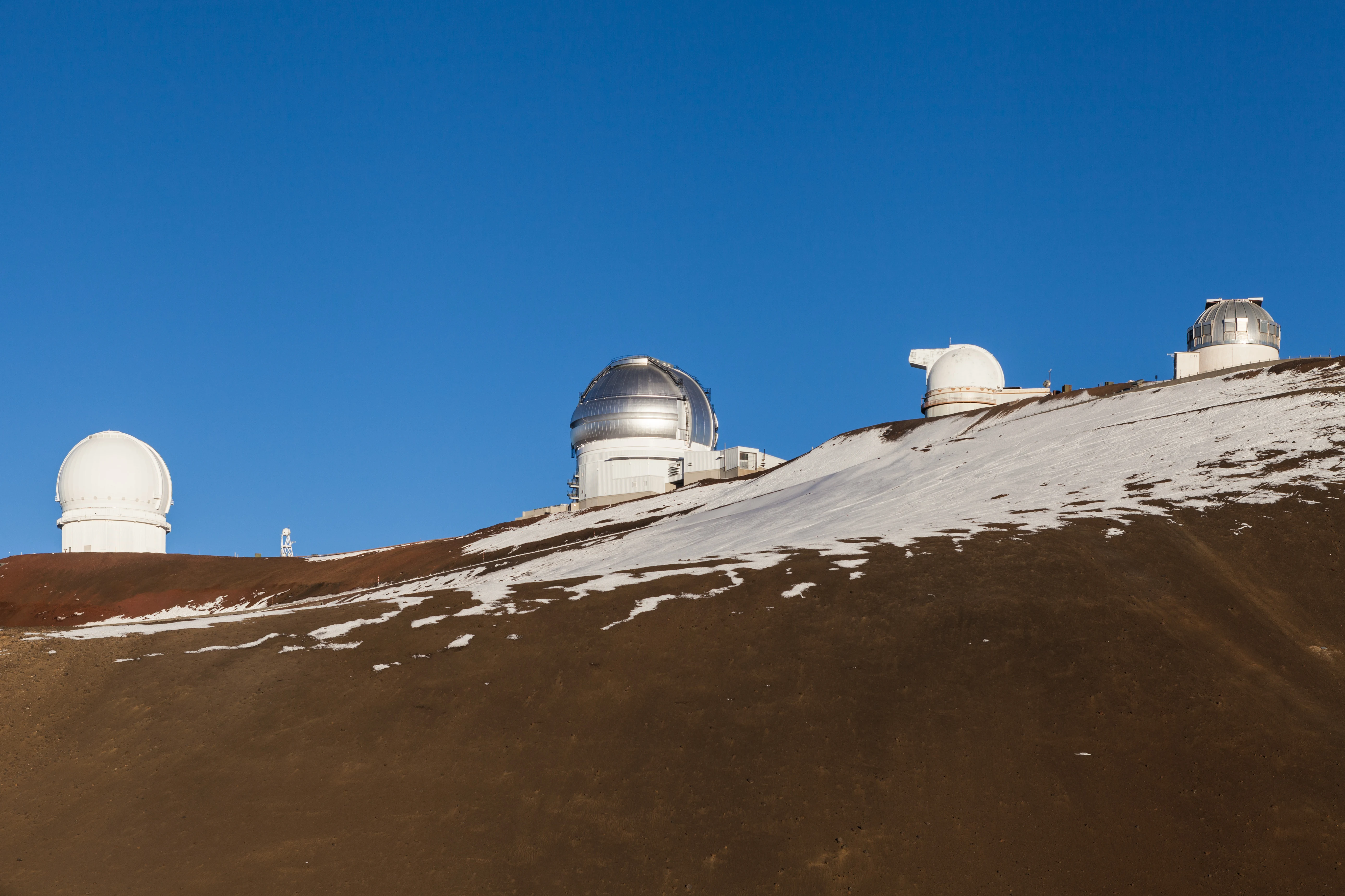
A team from the Observatoire de la Côte d’Azur and SISSA trained four machine-learning models on fifteen years of seeing measurements from the summit of Maunakea, then asked each one to forecast the next two hours of atmospheric turbulence. The winner, a long short-term memory network (LSTM), tracked the real seeing with a correlation of 0.965 ten minutes ahead, 0.759 at one hour and 0.672 at two hours. A second model, a normalizing flow called FloTS, came close to that accuracy, with at most 9% more error at any horizon, while also giving a full probability distribution for every forecast step. If you’ve ever stood next to a planetary rig wondering whether the air will settle before Jupiter sinks into the murk, that distribution is the part to care about.
The paper is arXiv:2610.29654 by Mary-Joe Medlej, Rahul Srinivasan, Simon Prunet, Aziz Ziad and Christophe Giordano, posted on 21 October. It’s a nine-page proceedings paper for the SPIE Astronomical Telescopes + Instrumentation 2026 conference, so treat it as a benchmark report rather than a refereed journal result.
What “seeing” is, and how Maunakea measures it
Seeing is the blur that atmospheric turbulence adds to a star image. Pockets of air at slightly different temperatures bend light by slightly different amounts, so a point source smears into a dancing blob. Astronomers quote it as the full width at half maximum of that blob in arcseconds (1 arcsecond is 1/3600 of a degree). Lower is better. I’ve written before about how balcony heat wrecks planetary views in Nicosia regardless of aperture. That’s seeing.
The training data comes from the Maunakea Weather Center and was recorded by a combined MASS/DIMM monitor. A DIMM (differential image motion monitor) puts two small sub-apertures on one telescope and watches how the two images of the same star jitter relative to each other. Shake from the mount or wind on the tube moves both images together and cancels out. What’s left is atmospheric, and its variance converts directly into a seeing value. The MASS (multi-aperture scintillation sensor) measures twinkling to split the turbulence into altitude layers. The authors used the DIMM numbers, which integrate the whole column of air above the summit.
The raw series runs from September 2009 to November 2024 at 90-second sampling, with seeing values between 0.04″ and 5″. The team split it into continuous observing stretches, patched gaps, and resampled onto a 10-minute grid. That smooths out flicker nobody could act on anyway.
This kind of forecast is called nowcasting. Services like Meteoblue’s seeing forecast, the one I lean on for Troodos trips, run weather models hours to days ahead. A nowcast takes the seeing measured over the last couple of hours and extrapolates the next couple. It knows nothing about the jet stream. It only knows the recent shape of the curve.
Four models, one setup
Every model got the same job. Take 2 hours of history (12 points at 10-minute spacing) and predict the next 2 hours (another 12 points). The authors report that longer input windows didn’t improve anything in their early tests.
- A plain recurrent neural network (RNN), the baseline. It reads the sequence one step at a time and carries a hidden state forward. Plain RNNs are notoriously bad at holding on to information over many steps.
- An LSTM, the same encoder–decoder layout but with gated memory cells that decide what to keep and what to forget. One encoder layer, two decoder layers, 100 hidden units each, dropout of 0.3, trained with the Adam optimizer at a learning rate of 10⁻⁴ on mean squared error.
- A Gaussian process (GP) with an exponential kernel, where correlation between two moments decays exponentially with the time between them. GPs give you an uncertainty band for free, but fitting one costs time that grows with the cube of the training-set size, so the authors fitted the hyperparameters on random subsets of 500 training pairs.
- FloTS, a normalizing flow. A flow learns an invertible transformation that turns a simple Gaussian into whatever shaped distribution the data actually has. This one is a masked autoregressive flow conditioned on an LSTM encoder that reads the 2-hour history (they tried linear, fully connected, RNN and GP encoders, and the LSTM worked best). The output is a full probability density for each future step instead of a single number.
The numbers
Here are four of the twelve forecast horizons, read from the paper’s Figure 1. Each cell gives the RMSE (root mean square error, lower is better) with the Pearson correlation in brackets (higher is better).
| Horizon | RNN | LSTM | GP | FloTS |
|---|---|---|---|---|
| 10 min | 0.143 (0.828) | 0.062 (0.965) | 0.083 (0.954) | 0.064 (0.963) |
| 30 min | 0.171 (0.750) | 0.127 (0.848) | 0.148 (0.848) | 0.135 (0.825) |
| 60 min | 0.193 (0.682) | 0.160 (0.759) | 0.183 (0.765) | 0.164 (0.746) |
| 120 min | 0.218 (0.620) | 0.192 (0.672) | 0.218 (0.673) | 0.198 (0.645) |
The heatmap doesn’t label the RMSE unit. The seeing values plotted elsewhere in the paper are in arcseconds, so I read these as arcseconds too, but that’s my inference.
Some things I pulled out of the full grid:
The LSTM’s error grows about 3.1× between 10 and 120 minutes (0.062 to 0.192). Squaring the correlation gives the share of the variation the forecast explains: roughly 93% at 10 minutes, 58% at one hour, 45% at two hours. Ten minutes out, the forecast is very good. Two hours out, it’s catching the general drift and missing a lot of the detail.
FloTS’s RMSE is never more than 9% above the LSTM’s. The biggest gap is at 20 minutes (0.115 against 0.106), and from 50 minutes onward it’s only 2–5%. You pay very little in accuracy for getting a distribution instead of a point.
The plain RNN loses everywhere, and at 10 minutes its error is more than double the LSTM’s, which fits the textbook story about gated memory.
The GP is more interesting than the paper’s framing suggests. On RMSE it falls behind: 34% more error than the LSTM at 10 minutes, about 14% more at one and two hours, and by 120 minutes its error has climbed to 0.218, level with the plain RNN. But its correlation matches the LSTM at 30 minutes and is very slightly higher at 60 and 120 minutes (0.765 against 0.759, and 0.673 against 0.672). So the GP follows the ups and downs about as well, but its predictions sit further from the true values. One plausible reason: an exponential kernel pulls the forecast back toward the mean as the horizon grows, so it gets the shape right and the level wrong. The paper’s “combined score” averages normalized RMSE and correlation, and the authors report the LSTM winning it at nearly every horizon.
Why a distribution beats a single number
At the telescope, I don’t need “seeing will be 0.9″ at 23:40”. I need “what are the odds it stays under 1.5″ for the next 45 minutes, long enough to run a lucky-imaging sequence?” A point forecast can’t answer that. A predictive distribution can.
Seeing is also an awkward quantity for Gaussian error bars. It can’t go below zero, and its distribution is skewed, with a long tail toward bad values when a layer of turbulence rolls in. A symmetric band around the mean fits that badly. A flow can learn a lopsided or even two-peaked distribution if that’s what the data looks like, and the authors argue that’s FloTS’s main advantage over the GP.
Raw FloTS came out underconfident: its predicted spread was wider than the real scatter. The fix was post-hoc temperature scaling, the same trick Guo et al. (2017) popularized for overconfident image classifiers. You raise the density to a power, 1/T. A temperature above 1 widens the distribution and below 1 sharpens it. Here T varies with the coverage level and is fitted as a polynomial so that, for example, the 68% region really contains the truth 68% of the time on validation data. In the example forecast the paper shows, calibration tightens the density around the observed seeing curve without shifting its centre.
What the proceedings don’t show
As someone who spent years shipping time-series models, I’d want a few more things before calling this operational.
There’s no persistence baseline. The forecast “seeing two hours from now equals seeing right now” is the bar every nowcast has to clear, and on a stable night it’s hard to beat. The table compares models against each other, not against that.
The calibration result is shown as one example night. The abstract mentions probabilistic metrics, but the paper doesn’t print a calibration score or a coverage figure for the test set as a whole. One well-behaved example doesn’t tell you how the uncertainty holds up on bad nights.
The train/test split isn’t described in detail. With overlapping sliding windows on a time series, a random split can leak near-identical samples between training and test and flatter every model. A chronological split (say, train on 2009–2020, test on 2021–2024) would rule that out. The paper may well have done this, but it doesn’t say.
It’s one site with one input variable. The model sees only past seeing, with no wind, temperature or humidity; the authors list both gaps as future work. Maunakea is a 4,200 m summit surrounded by ocean, so how this transfers to a continental site, let alone a rooftop, is an open question.
I couldn’t find a code release linked from the paper or the arXiv page.
None of this makes the result wrong. It makes it a clean first benchmark, which is what a proceedings paper is for.
What it means if your observatory is a balcony
For my own setup, the honest answer is “not much, directly”. The Seestar S50 has a 50 mm aperture. Its Dawes limit, the finest double star it can split, is about 116/50 ≈ 2.3″, and its pixels each cover about 2.4″ of sky (2.9 µm pixels at 250 mm focal length). On most nights the atmosphere isn’t what limits that little scope. Seeing starts to cost you with a 150–250 mm aperture on planets, where good nights give sharp detail and bad nights give mush.
The two-hour horizon also doesn’t help with the decision I actually agonize over, which is whether to drive to Troodos. That’s a 90-minute drive from Nicosia, which uses up most of the forecast window before I’ve unfolded a tripod. Go/no-go is still a job for weather-model forecasts like Meteoblue’s. A nowcast fits the on-site decision: whether to start a planetary capture run now or wait 40 minutes for things to settle. For the Mars–Jupiter conjunction on the morning of 16 November, that’s exactly the call I’ll be making by hand.
The catch is that a nowcast is only as local as its sensor. The MASS/DIMM sees the air above a summit, and the turbulence that ruins my balcony nights is the few metres of warm air coming off the building. Nothing on Maunakea knows about that. To nowcast your own site you’d need your own seeing series. The closest thing most of us have is the star size our capture software logs frame by frame. N.I.N.A., for example, records an HFR (half-flux radius) for every sub. That’s a noisy proxy, mixed up with focus drift and guiding, but it’s a time series of your own sky. The model in this paper is small: a few layers with 100 units each, fed 12 numbers to predict 12 more. Training something like it on a season of your own logs is a weekend project.
I’d put the result like this. Ten minutes ahead, ML seeing nowcasts are already very good. One to two hours ahead, they explain about half the variation, which beats guessing but isn’t something to bet a night on alone. The flow model’s distribution is the part I’d want in an observatory scheduler, and the part I’d most like to see checked on more than one night and more than one mountain.