At the end of May 2023, a few days into LIGO’s fourth observing run, the Hanford detector started throwing out a new kind of noise: a narrow line near 589 Hz, lasting less than 0.4 seconds. The neural network that had sorted LIGO’s glitches since 2017 looked at 267 of them and called them “Whistle”, with an average confidence of 0.976. That was wrong, and the network was sure of it. A replacement classifier, built by the Gravity Spy team, looked at the same events and shrugged. It split them across three classes, with confidence scores between 0.35 and 0.46. For a model that only knows 23 categories, that kind of hesitation is the right answer to a glitch it has never seen. It’s since been identified as a new class, discussed on the project’s volunteer forum under the plain name “589 Hz”.
That replacement is described in Wu et al., arXiv:2401.12913, published in Classical and Quantum Gravity in 2025. The authors write that it has been running in the Gravity Spy pipeline during O4, used by volunteers on Zooniverse and by LIGO’s detector experts. It’s a good case study in a problem I spent years on in industry: a classifier whose most useful output is knowing when it doesn’t know. It’s also timely. The LIGO–Virgo–KAGRA observing plan put the start of a six-month Intermediate Run 1 between late October and mid-November 2026, with both LIGO detectors taking part.
What a glitch is
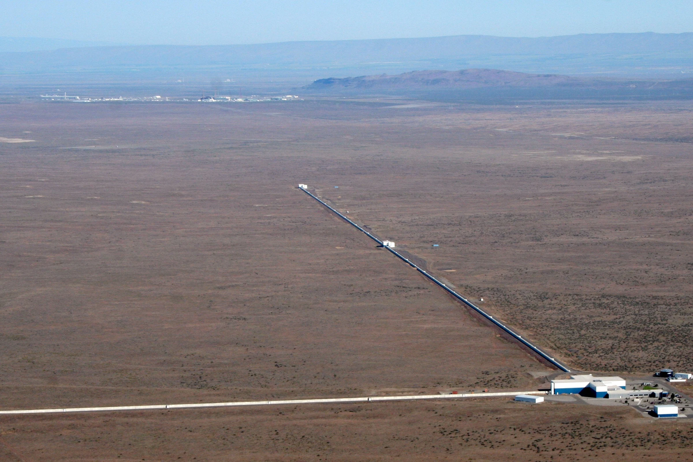
LIGO’s two detectors, in Hanford, Washington and Livingston, Louisiana, are L-shaped laser interferometers with 4 km arms. A passing gravitational wave stretches one arm and squeezes the other by a fraction of a proton’s width. An instrument that sensitive also picks up seismic rumble, wind, mains electricity, vibrating mirror suspensions and stray laser light bouncing off anything that moves. A glitch is a short burst of that noise, lasting from a fraction of a second to a few seconds. It can mimic a real signal, or land on top of one and corrupt it. I covered the GWTC-5.0 catalog in July; an event only gets into that list if the odds that it’s astrophysical, rather than noise, are at least 50%. Knowing what the noise looks like is half of that judgement.
Astrophotographers know a version of this problem: satellite trails, hot pixels, the frame smeared by a gust on the balcony. I wrote in October about how neural networks find satellite trails in survey images. LIGO’s job is the same in a different domain. Spot the junk, name it, and trace it back to the hardware so engineers can fix it at the source.
How a glitch becomes a picture
A pipeline called Omicron scans the detector’s output for bursts of excess power. Gravity Spy keeps only triggers with a signal-to-noise ratio above 7.5 and a peak frequency between 10 and 2048 Hz: loud enough to matter for gravitational-wave searches, and in the band where the searches look.
Each surviving trigger becomes a set of Omega scans, spectrograms with time on the horizontal axis, frequency on the vertical, and colour for loudness. They’re made with a constant-Q transform, which uses short time slices at high frequencies and long ones at low frequencies. Every glitch gets four of them, centred on the trigger, with windows of 0.5, 1, 2 and 4 seconds. The four windows exist because glitches come in very different lengths. A Blip is a short vertical teardrop. A Whistle is a sweeping V or W that takes much longer to play out. Repeating Blips only reveal themselves as repeats in the longer windows.
The 23 classes in the training set have names like a children’s book: Koi Fish, Paired Doves, Tomte, Helix, Scratchy, Wandering Line. A few name causes (Air Compressor, Power Line, Violin Mode, after the resonance of the fibres that hang the mirrors). Most describe shapes, agreed between LIGO scientists and volunteers.
Volunteers and machines, labelling each other
Gravity Spy started in 2016, after LIGO’s first observing run, and runs on Zooniverse. According to the new paper, more than 30,000 volunteers have made over 7 million glitch classifications. The loop runs both ways. Volunteer labels train the network. The network’s confidence scores, in turn, shape what volunteers see. The 2017 design paper describes newcomers moving through levels that add more glitch classes as they go, with the machine’s most questionable calls fed back to humans for a closer look. The classifier added in 2017 was retrained as new classes turned up, but its architecture barely changed.
The paper lists three faults with that original model:
- Early fusion. The four time windows were tiled into one 2×2 image and fed to a single network. To fit, each window was shrunk to 140×170 pixels, losing detail. Tiling also treats all four windows as equally informative, when a Repeating Blip may only show in the 4-second view.
- A shallow network. A few convolutional layers and fully connected layers. In a spectrogram, position carries meaning. A line at the top of the image and a line at the bottom are different glitches at different frequencies, unlike a cat photo, where a cat is a cat wherever it sits.
- Overconfidence. The old model gave confidences near 1.0 for almost everything, including its mistakes. That misleads volunteers and experts alike, and it hides new glitch types, because a new type should look like an uncertain prediction.
The new architecture
The replacement keeps the four windows apart until late in the network. The authors call this intermediate fusion.
Each window, resized to 448×448 pixels, goes through its own branch. Every branch has the same layout: convolutional blocks alternating with inception-residual blocks. Each of those runs 1×1, 3×3 and 5×5 convolutions in parallel to catch features at several scales, then adds the result back onto its input through a skip connection (the Inception-ResNet design from Google). Skip connections let a deeper network train without its gradients fading away. Each branch ends by squeezing its window down to a 128-number summary.
Then comes the part I like best: a gated attention module. It looks at the four 128-number summaries and assigns each a weight, with the four weights adding up to 1. The weighted average goes to a final layer that outputs probabilities for the 23 classes. The weights are a by-product you can read: they tell you which time window drove each decision.
The training tricks deal with noisy labels, lopsided classes and overconfidence:
- Label smoothing. Instead of “this is 100% a Blip”, the target is softened to slightly less than 1 for the right class, with the remainder spread over the others. The best smoothing parameter was β = 0.3; anything up to 0.5 beat no smoothing.
- Class weights inversely proportional to how common each class is, so rare classes aren’t drowned out.
- L2 regularization, dropout and early stopping (patience of 10 epochs), with the Adam optimizer at a learning rate of 2×10⁻⁵.
The training data is O3 glitches from Hanford and Livingston. To keep mislabelled examples out, the team only used glitches where volunteers and the old classifier agreed with a consensus confidence above 0.9. That was 84.5% of the dataset. They split it into 8,439 glitches for training, 1,687 for validation and 3,538 for testing. Every experiment was run five times with different random initialisations.
The numbers
All figures are means over five runs on the same O3 test set. To make the comparison fair, the old architecture was retrained from scratch on the same data.
| Model | Accuracy | Precision | F1 | AUC |
|---|---|---|---|---|
| Previous classifier (retrained) | 0.906 | 0.913 | 0.904 | 0.937 |
| Early fusion (windows tiled, one network) | 0.911 | 0.918 | 0.901 | 0.939 |
| Late fusion (four models, outputs combined) | 0.922 | 0.920 | 0.901 | 0.940 |
| Intermediate fusion, max pooling instead of attention | 0.916 | 0.928 | 0.908 | 0.948 |
| Intermediate fusion + gated attention (deployed) | 0.941 | 0.950 | 0.931 | 0.965 |
The overall gain is 2.7 to 3.7 percentage points depending on the metric, and every headline comparison against the deployed model passed the authors’ significance test (p < 0.05). The overall numbers hide the more interesting part. Per class, the biggest jumps in accuracy are in the hard, rare classes:
- Wandering Line: 0.520 → 0.740
- Helix: 0.732 → 0.891
- Repeating Blips: 0.772 → 0.933
- Low-frequency Lines: 0.818 → 0.916
- Scratchy: 0.862 → 0.957
Wandering Line had only 25 training examples and 25 test examples. Going from 0.52 to 0.74 on 25 glitches means about 13 correct becomes 18 or 19. That’s real progress, but it’s a small sample, and 0.74 is still the weakest class in the table. The new model did slightly worse on two classes, Koi Fish (0.921 → 0.917) and Scattered Light (0.929 → 0.924), and neither difference was significant. Both overlap with similar-looking classes: a very loud Koi Fish resembles an Extremely Loud glitch, and Scattered Light shares the low-frequency, long-duration look of Low-frequency Lines.
What the attention weights show
The attention weights match what experienced volunteers do by eye. For Repeating Blips, the model leans on the 2- and 4-second windows, where the repetition shows up. For a single Blip or a Koi Fish, it weights the 0.5-second window, where the short burst is resolved. For “No Glitch” it relies most on the 4-second window: confirming that nothing is there means checking the widest view. Whistles get most attention at 2 seconds, long enough to show both the sweep shape and the repeated sweeps that real Whistles often have.
That tells you which window mattered. It doesn’t tell you which pixels; the authors list a pixel-level method (Grad-CAM) as future work.
Calibration: how sure is “sure”?
A classifier is well calibrated if, among all the glitches it labels “Blip” with 40% confidence, about 40% really are Blips. The paper measures this with the expected calibration error (ECE), the average gap between stated confidence and actual accuracy. The old model’s ECE was 0.09 and the new one’s is 0.06. The reliability plots show both models are still overconfident, the new one less so, especially at confidences above 0.8.
The more telling test used 2,267 real glitches from early O4, between 24 May and 19 September 2023, when some glitch types looked different from their O3 versions. The old model still reported confidences close to 1 for nearly every class. The new model stayed confident on Extremely Loud and Low-frequency Lines, whose shapes hadn’t changed much, and dropped its confidence for Whistle, Wandering Line, Violin Mode and Scratchy, whose O4 versions looked different. That’s what you want from a model meeting unfamiliar data: low confidence wherever the world has changed.
The 589 Hz glitch is the clearest example. The old model’s confident “Whistle” (0.976 ± 0.059) became, in the new model, 195 events labelled Whistle at 0.463 confidence, 49 labelled No Glitch at 0.428, and 23 labelled Violin Mode at 0.347. None of those labels is right, because no right label existed yet. The low scores are what make the cluster stand out for a human to look at.
My read, as someone who has shipped classifiers
A few things to keep in mind before taking 0.941 at face value.
The test set is the easy part. The training and test sets were both filtered to glitches with consensus confidence above 0.9. The remaining 15.5%, where volunteers and the old model disagreed or were unsure, is exactly where a better classifier would matter most, and it isn’t measured here. The authors say a test set checked by LIGO’s detector-characterization experts is future work.
The labels came partly from the old model. Ground truth came from volunteers plus the previous classifier. The new model is partly being scored on how well it agrees with its predecessor’s confident calls. That can’t be avoided at Zooniverse scale, but it does cap how far a successor can visibly improve.
It can’t name new things. It’s a 23-way supervised classifier. When a new glitch type appears, the best it can do is be unsure. Humans still have to spot the cluster, name it, and retrain. The paper presents that as the design: the model flags, volunteers investigate.
Good engineering choices. Retraining the baseline on the same split, reporting the spread over five runs, testing significance and measuring calibration are all things I’d want in any ML paper, and plenty of astronomy ML papers skip some of them. The paper points to the Gravity Spy pipeline code on GitHub, and the volunteer and ML classification data sit on Zenodo.
What it means for you
This is AI × astronomy you can do from the sofa on a cloudy night. Gravity Spy is open on Zooniverse. You start with a handful of classes and get more as you level up. According to the project page, volunteers are now also asked to look at extra detector data to help trace glitches to their causes. Every label you make feeds the next training set.
If the Intermediate Run keeps to the published schedule, fresh glitches will be coming off the detectors this month, along with public gravitational-wave alerts. The ones that matter to observers are neutron-star mergers, which can produce a visible kilonova. Deciding whether a candidate is a real signal or noise depends on knowing the noise, and that knowledge is what all those sorted Koi Fish and Blips add up to.
From my balcony, the closest I come to this is flagging bad subs before a stack. The lesson I’d take from the paper is the one I’d give any team shipping a classifier: accuracy gets the headlines, but calibration is what lets you notice something new.